Modelling Outbreaks
As the world is emerging from waves of Coronavirus infections and facing new threats of virus outbreaks, the scientist in us may ask: how can we model such outbreaks? One common approach is to use so-called “compartmental models”, and in particular the SIR-model. Here, the individuals of the population fall into one of the following three categories: Susceptible, Infected or Recovered.
Susceptible individuals can become infected upon contact with infected individuals. Infected individuals may either infect susceptible individuals or recover. The recovered individuals stay recovered and cannot become infected again (*). If we use the variables S, I, and R to denote the number of individuals in each category, then, under some simplifying assumptions to make the model tractable, the expected values of these variables at the next (t+1)-st time step are given by:
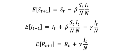
Here N is the size of the whole population, β is the infection rate, γ is the recovery rate, and initially I₀ is very small (but positive), S₀=N-I₀, and R₀=0. The above equations can be viewed as discretization of the differential equations describing the time-continuous version of the model.
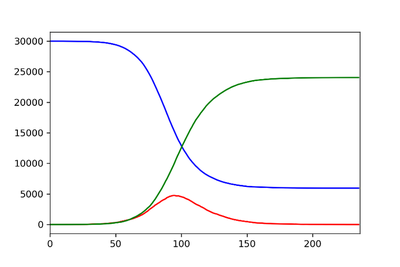
The spread of the infection has a logistic growth: at the beginning it grows exponentially until a large fraction of the population is infected. From that, the growth rate starts to decrease until herd immunity takes over and the infection vanishes. See Figure 1, where the plot of Rₜ – the number of individuals who have been infected by time t – is a logistic curve.
This model is a key element of our recently published work, where we studied two questions:
- Will the disease die off before any significant number of individuals get infected, or will it take root and spread until the population reaches herd immunity?
- Is travelling always making the spread of the virus worse?
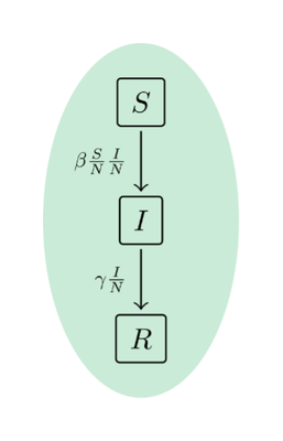
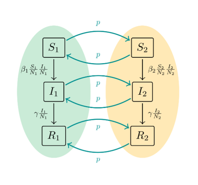
To answer the first question, we model the individuals as agents and assign a certain probability to every state transition, as illustrated in Figure 2. In expectation, one step of this discrete-time model is described by the above equations. However, any given infected agent may infect more or fewer other agents than expected, or it may remain infected for a shorter or longer time than expected. When we take that into account, we capture the scenarios when the disease is extinguished early in the process. We calculate the exact probability with which this happens. Modeling this behaviour leads to a more precise prediction of the expected spread of the disease than what we obtain from the differential equations.
For the second question, we assume there are multiples countries, which have their own, potentially different, infection rates β₁,β₂,…, but the same recovery rate γ. Figure 3 shows the transition diagram for the case of two countries, where the arrows with label p represent traveling and larger p means that traveling is more frequent.
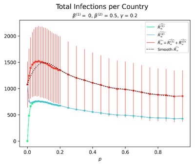
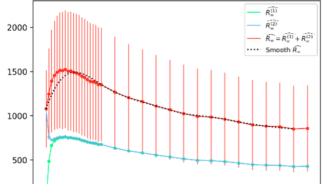
Our simulation results indicate that, in some cases, travelling would decrease the total number of infections across countries. Consider, for example, two countries with β₁=0, β₂=0.5 and the common γ=0.2. Whenever the recovery rate is larger than the infection rate (the first country would be the extreme example of this), the total number of infections decreases very quickly. Now, by allowing travelling between countries, some sort of mixing and averaging happens and the total spread of the disease across both countries may increase or decrease. For this example, Figure 4 shows that the average R∞ – the final spread of the disease measured as the total number of individuals who have ever been infected – first increases with increasing p, but then decreases. For p=1 (high level of traveling), the total spread of disease is actually smaller than for p=0 (no traveling).
Should you use this research to advocate trips around the world to “save the planet”? Probably not, since even if this could theoretically decrease the global spread of the infection, the price would be an inevitable increase of the infection in the places with small β. But it would surely be an interesting conversation starter with fellow travelers at airport terminals.
(*) In the context such as COVID-19, in which it is known reinfection is possible, the SIS model can be more accurate.
The above article refers to the work “On Early Extinction and the Effect of Travelling in the SIR Model”, by Petra Berenbrink, Colin Cooper, Cristina Gava, David Kohan Marzagão, Frederik Mallmann-Trenn and Tomasz Radzik. This work was recently published at the UAI 2022 - Association for Uncertainty in Artificial Intelligence Conference.
Read more about the project here.
